graph BT
    A(["<strong>base R</strong>
Rの基本構文・関数
例: mean(), sum(), if"]) -->
    B(["<strong>modern R</strong>
便利な文法・スタイル
例: |> パイプ, tibble, dplyr 文法,<br> ggplot2 文法"]) -->
    C(["<strong>Packages</strong>
Rに追加するツール集
例: tidyverse, ggplot2,<br>readr, shiny"])


%% ノードのスタイル
style A text-align:center
style B text-align:center
style A text-align:center, fill:#FFD700,stroke:#333,stroke-width:1px,font-weight:bold;
style B text-align:center, fill:#87CEFA,stroke:#333,stroke-width:1px,font-weight:bold;
style C text-align:center, fill:#90EE90,stroke:#333,stroke-width:1px,font-weight:bold;
初心者向けR Studioの使い方
Rを用いて学ぶ量的テキスト分析講習会
苅谷千尋 
金沢大学
November 2, 2025
自己紹介:レトリックの受容史
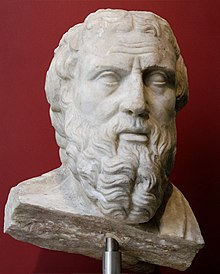
プルタルコス
民衆が演説をどう受け止めるかに関心を持たない者は、すなわち寡頭制を支持する者、説得よりも暴力に頼ろうとする者である。
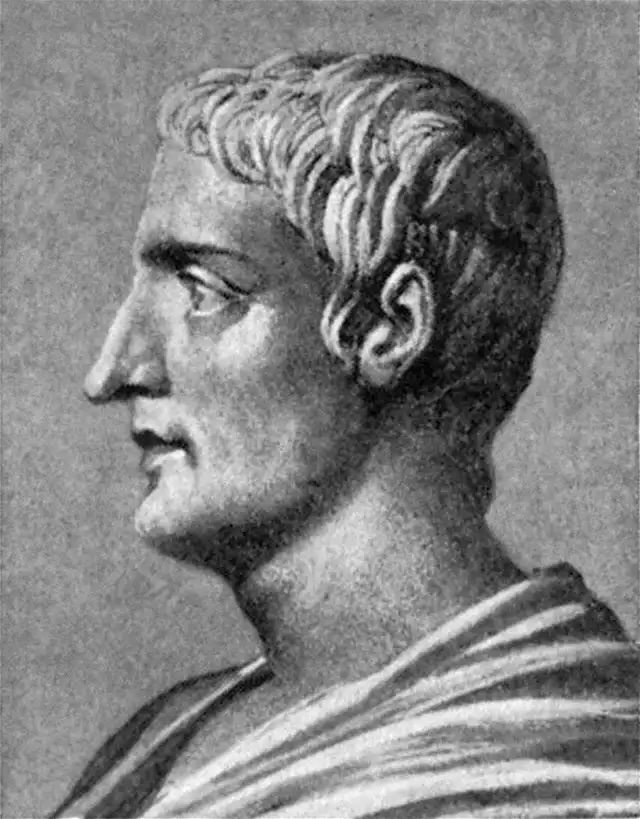
タキトゥス
今昔を比較して暇を潰す老人らは、つぎのことに気がついた。国家を統治した歴代の元首のうちで、他人の雄弁術を必要としたのは、ネロが最初であると。
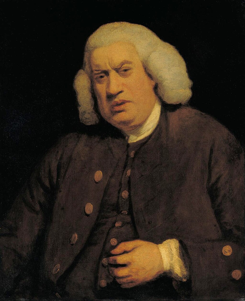
自己紹介:レトリックの受容史 / 議会ジャーナリズム
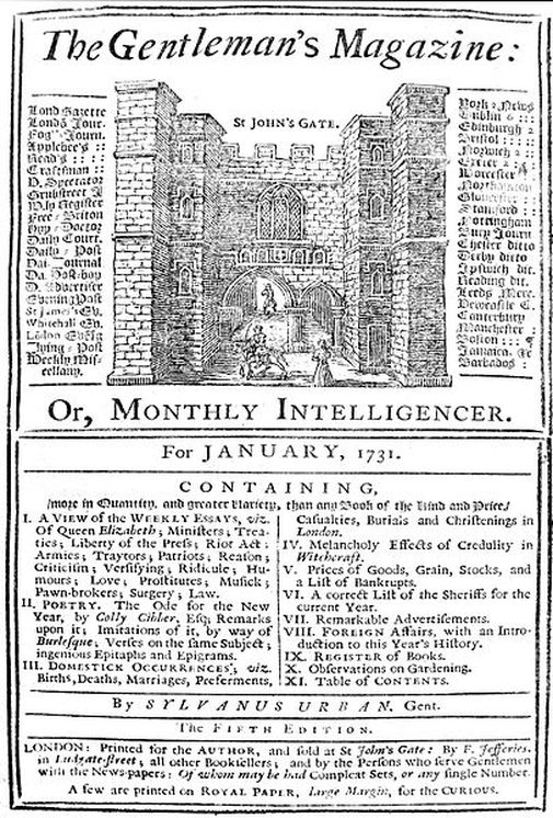
サミュエル・ジョンソン(The Gentleman’s Magazine)
最後に演説された貴族議員〔Hurgo院Heryef卿〕はあまりに偉大な雄弁の達人です。その巧みさゆえに、人は、彼の言葉を聞くに当たって、喜びから自然に生まれるあらゆる注意力を向けることがありません。聴き手の心には、部分的な表現や巧みな推論に惑わされるのではないか、という恐れから不安が生じるものです。しかし、彼はこのようなあらゆる不安を生じさせないほどに恐ろしい、理路整然と論じられる人(reasoner)なのです。諸君、私が常に恐れているのは、この貴族議員の想像力が与える装飾(ornaments)のなかで、誤謬が真実であるかのように見えすぎてしまうことなのです。そしてまた、理性の光によって導かれる自分自身を想像しながらも、その詭弁(sophitry)が私の知性(understanding)を惑わすことなのです。諸君、そこで私は、彼の装飾を再検討し、それが真実の力によるものなのか、それとも雄弁によるものなのか、私は試してみようと思う。
自己紹介:レトリックの受容史 / 議会ジャーナリズム
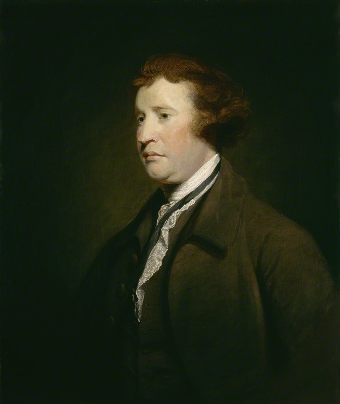
エドマンド・バーク
ある古代の著述家(プルタルコスだと思う)は、「聴衆の心に刺を刺した唯一の雄弁家」と呼ばれるペリクレスの雄弁について、幾つか詩を引用している。ペリクレスと同様に、この声明の雄弁さは、真の人間性(humanity)の感性と矛盾せず、むしろ感性を強化するものであり、私の心には皮膚以上に深く刺さった刺が残っている。この刺は、殺人者が外科であらゆる手を尽くして取り除こうとしても取り除くことはできず、また、この刺が生み出した胸の高鳴りは、強奪や没収という皮膚を和らげる湿布薬をもってしても和らげることはできない。私はこの〔革命フランス〕共和国を愛すことができない。
基礎:なぜRなのか / なぜQuartoなのか
5. 簡易的な記述法(Quarto)
| 要素 | Markdown構文 | 例 |
|---|---|---|
| 見出し | # H1## H2 |
H1 見出し H2 見出し |
| 太字 | **bold text** |
bold text |
| イタリック | *italicized text* |
italicized text |
| 引用 | > blockquote |
> blockquote |
| リンク | [金沢大学](https://www.kanazawa-u.ac.jp) |
金沢大学 |
| 画像 |  |
色や文字の大きさは、別途、CSSファイルを用意して、変更する必要があります
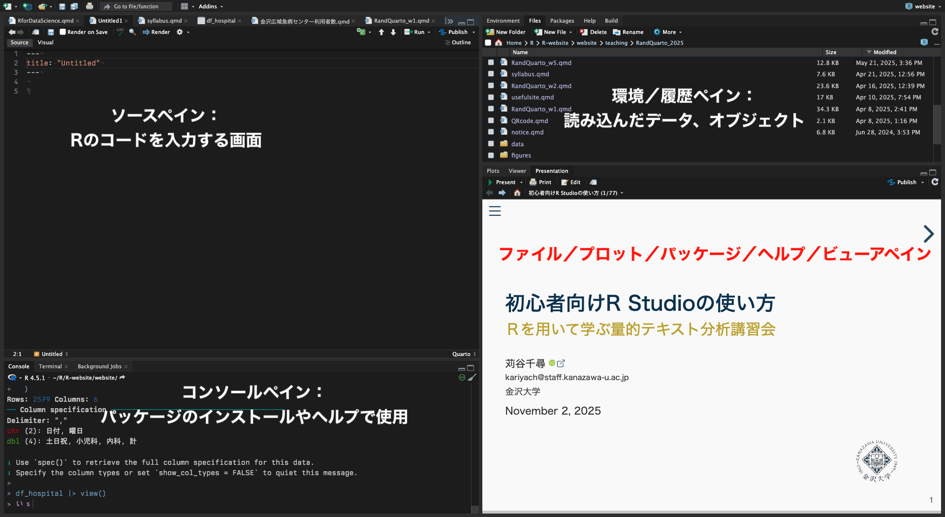
準備:R Studio(ペイン)の見方
- 4画面構成
- 主要な操作は左上のソースペインで行う
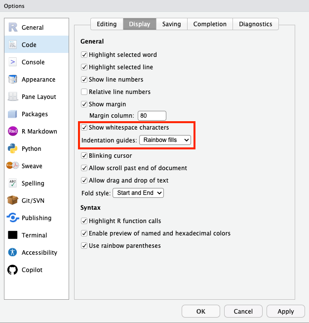
準備:R Studio(ソースペイン)の外観の変更
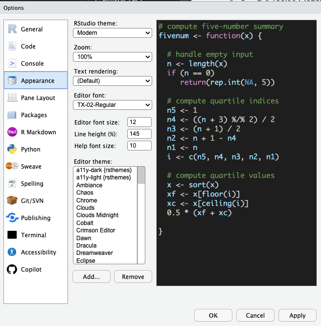
準備:R Studio(ソースペイン)の外観の変更
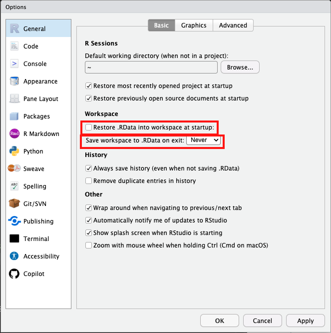
準備:R Studioの保存・復元設定
- 意図しない古いデータが使われることを避ける必要があります
8. 「.RData」保存をオフにする
- メニュー > Tools > Global Options > General > Workspace
- Restore .RData into workspace at startup: チェックを外す
- Save workspace to .RData on exit: Neverを選択
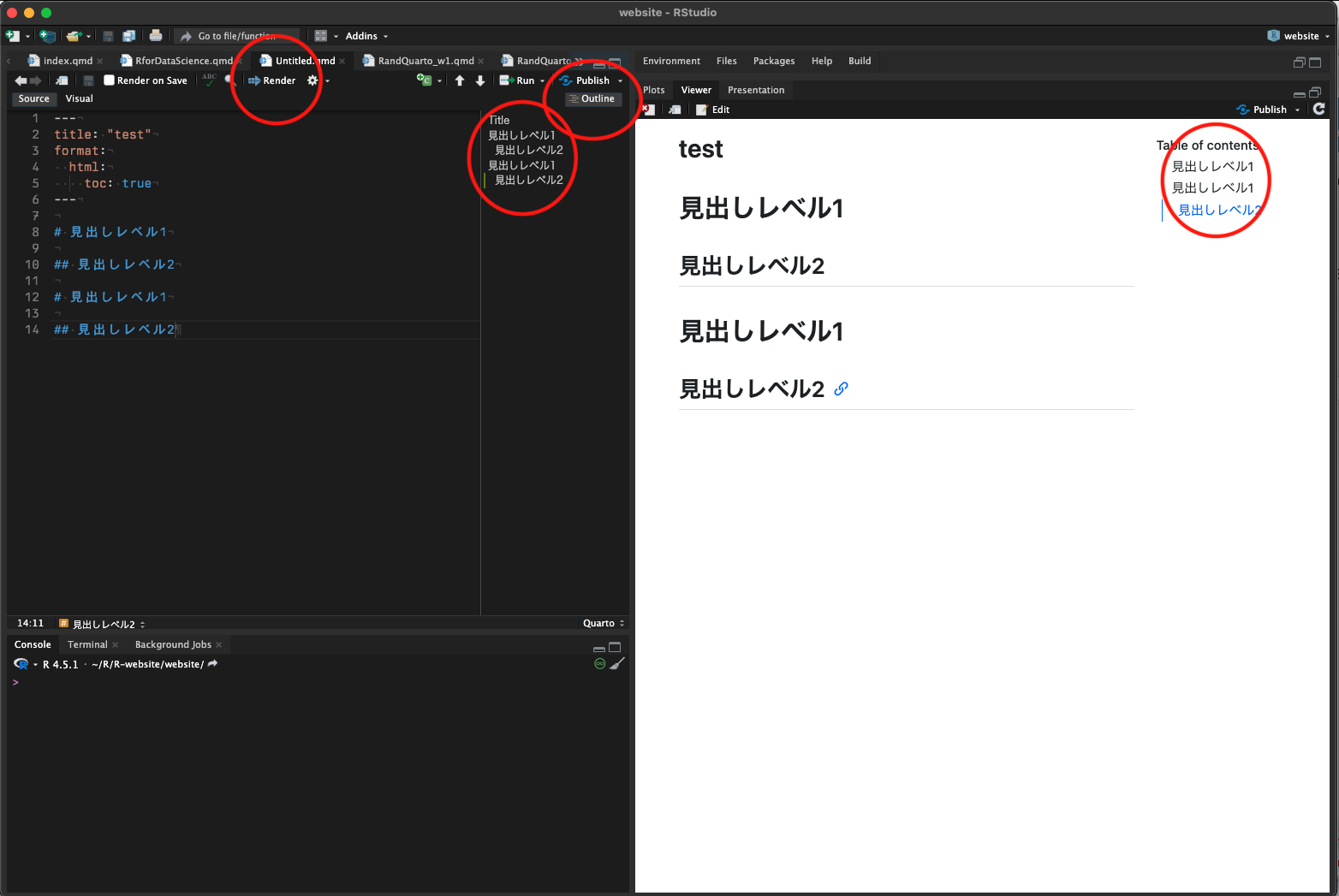
準備:目次の追加(YAML)
- Renderをクリック
- YAMLで設定している出力形式に従って右下のペイン(Viewer/Presentation)にレポートが出力される(全てのR Chunkが実行される(後述))
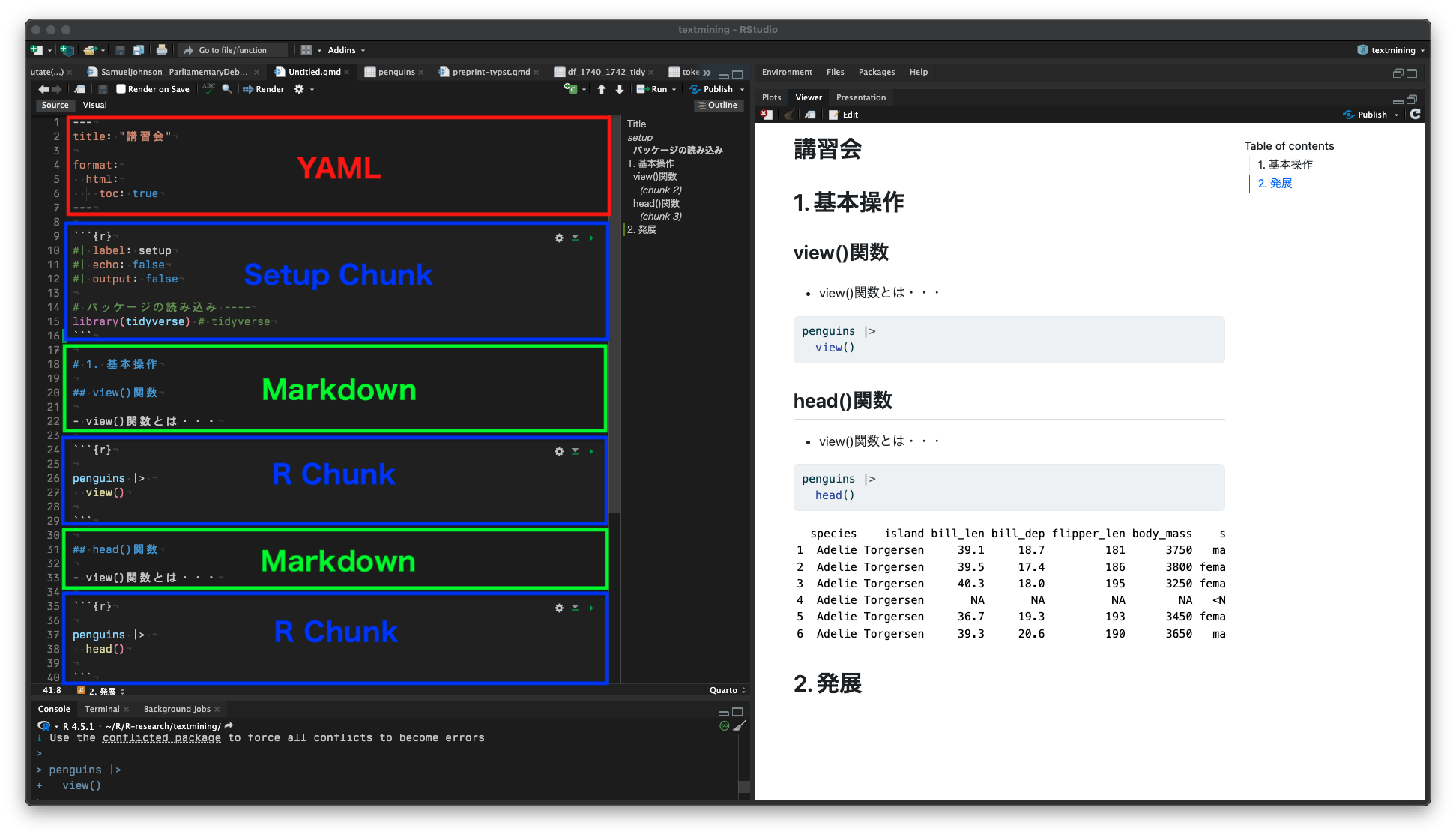
準備:Quartoファイル
基本:データセット
- パーマーランド(南極)の3つの島に住むペンギンたちのデータ(Allison Horstさん作成)
ペンギンの種類:
- Adelie(アデリーペンギン)
- Gentoo(ジェンツーペンギン)
- Chinstrap(ヒゲペンギン)
島の名前:
- Biscoe(ビスコー)
- Dream(ドリーム)
- Torgersen(トージャーセン)

基本:データの型
データの型
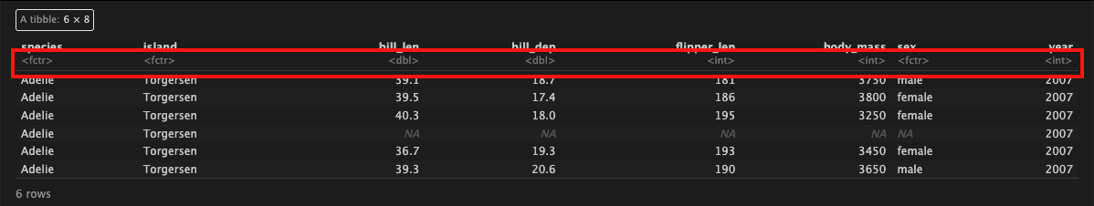
基本:データフレームの型
データフレームの型
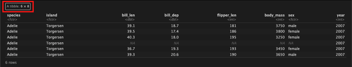
- tibble(ティブル)はtidyverseで使われるデータフレームの新しい形式
- base Rのデータフレームであるdata.frameを、より見やすく、扱いやすく改良したもの
- dplyrやggplot2などの関数と相性がよい
- tibbleは列にlistを入れられるので、グループごとのデータをまとめて操作する「ネスト処理」と相性がよい
- 文字列を自動的にfactorにしない、出力が見やすい(先頭だけを整形して表示)間などの特徴もある
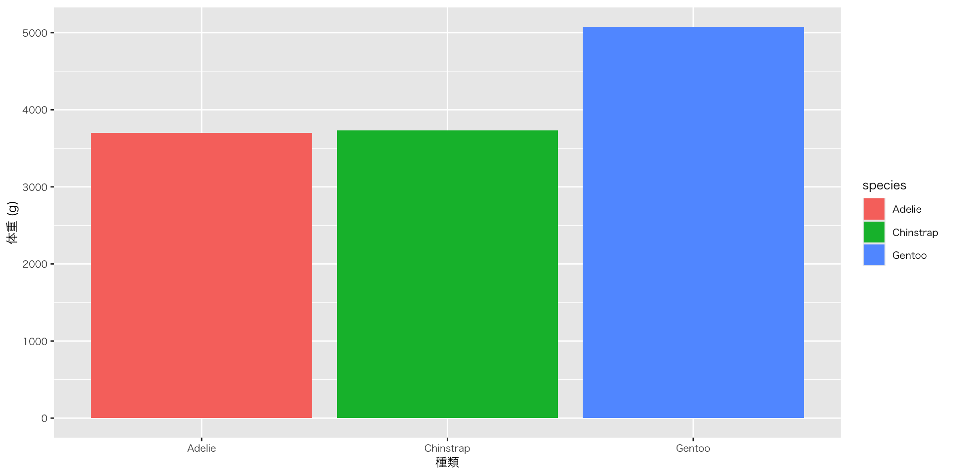
基本:作図
図を作る:ggplotに渡す前にデータを整形する
- group_by / summariseで集計した結果を、ggplotで図として出力する
ggplotはレイヤーを重ねて図を作ります。演算子がパイプと違って「+」なのは、要素の追加をイメージしているからです
penguins |>
  group_by(species) |>
  # summarise()関数: 元データを要約して新しい表を作る関数
  ## 第2引数で列を定義
  ### 計算結果(ここではmean()関数の結果)に列名mean_body_mass(任意)を付けて出力
  summarise(mean_body_mass = mean(body_mass, na.rm = TRUE)) |>
  ggplot(aes(x = species, y = mean_body_mass, fill = species)) + # fill = speciesは棒や面を塗りつぶす色をspeciesに応じて変える、の意
  geom_col() +   # geom_colはデータに渡されたyをそのまま棒の高さに使う
  labs(          # 変数名から任意のラベル名に変える
    x = "種類",
    y = "体重 (g)"
  )
基本:作図 > ggplotの日本語問題
ggplotの日本語問題

基本:作図
図を作る:ggplotに渡した後にデータを計算する

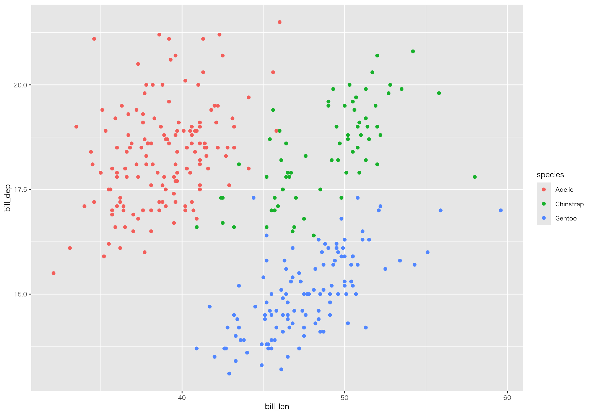
基本:作図 > 散布図
散布図の作成
基本:作図 > 棒グラフ(ファセット)
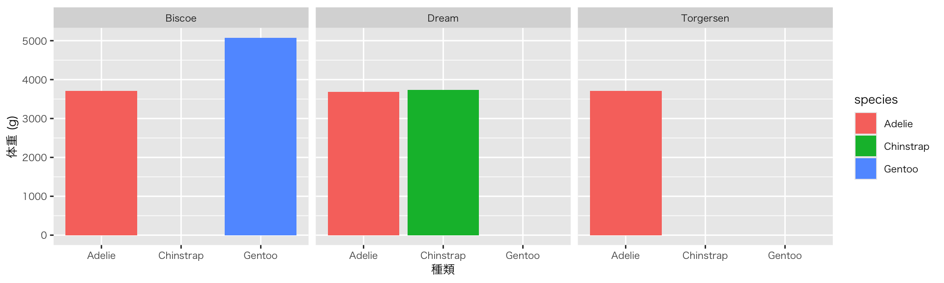
見比べる
- species(種)とisland(島)に関係はあるの?
- facet()関数:図を変数の値ごとに分割して、複数の小さなグラフにする
- 1つの大きなデータの面を切り分けて、それぞれの側面を並べて見る
基本:ショートカット
代入演算子(<-)のショートカット
- チャンク内で
- Win: Alt + 「-」キー
- Mac: Option + 「-」キー
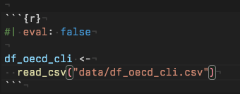
特定のチャンクが動かない
- 原因がすぐにわからないエラーが出ても安心です(よくあることです)
- そのチャンクだけ実行をスキップできるので、レポート全体のレンダーに影響しません(冒頭に「#| eval: false」と書く)
実践:URLからデータ取得(OECD景気先行指数)
- OECDデータセット:Composite Leading Indicators (CLI)
- urlを指定して、データを取得(ファイルはダウンロードしない)
url <- "https://sdmx.oecd.org/public/rest/data/OECD.SDD.STES,DSD_STES@DF_CLI/.M.LI...AA...H?startPeriod=2023-02&dimensionAtObservation=AllDimensions&format=csvfilewithlabels"

df_oecd_cli <- read_csv(url) # 指定したURLからデータを読み込む

# URLにアクセスできない場合(短時間にアクセスを繰り返すと接続拒否されることがあります。その場合は、エラーが出てデータを取得できません。以下のコメントアウトを外して(ハッシュタグを削除)、csvファイルからデータを読み取って下さい)
# df_oecd_cli <-
#  read_csv("data/df_oecd_cli.csv")

de_oecd_cli_selected <-
  df_oecd_cli |>
  select(REF_AREA, TIME_PERIOD, OBS_VALUE) |> # 必要な列を取り出す
  mutate(TIME_PERIOD = ym(TIME_PERIOD))  # 年月を日付型に変換

countries <- c("JPN", "USA", "DEU", "FRA", "KOR") #主要国だけ選ぶ(主要国のオブジェクトを作る)

de_oecd_cli_selected |>
  filter(REF_AREA %in% countries) |> # REF_AREA が countries に含まれる行だけを抽出
  ggplot(aes(x = TIME_PERIOD, y = OBS_VALUE, color = REF_AREA)) +
  geom_line()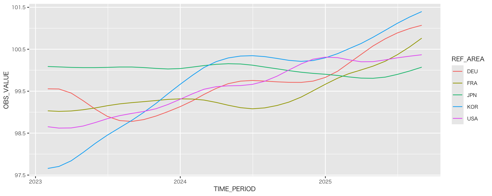
実践:URLからデータ取得(OECD景気先行指数)
見た目を整える
de_oecd_cli_selected |>
  filter(REF_AREA %in% countries) |>
  ggplot(aes(x = TIME_PERIOD, y = OBS_VALUE, color = REF_AREA)) +
  geom_line() +
  scale_x_date(
    breaks = scales::breaks_width("3 months"),  # x軸の間隔調整
    labels = scales::label_date_short()         # 年と月を行を変えて表記
  ) +
  scale_y_continuous(
    breaks = scales::breaks_extended(8),        # 目盛りの個数を指定
    labels = scales::label_number(accuracy = 1) # 数値表示(小数なし)
  ) +
  labs(                                         # ラベル名と凡例名の変更
    x = "Year",
    y =  "Composite Leading Indicator (CLI)",,
    color = "Country"
  ) +
  scale_color_paletteer_d("awtools::mpalette") + # 配色変更
  theme(axis.text.x = element_text(angle = 30, hjust = 1)) # x軸のラベルの傾き調整(この事例は適切なユースケースではない)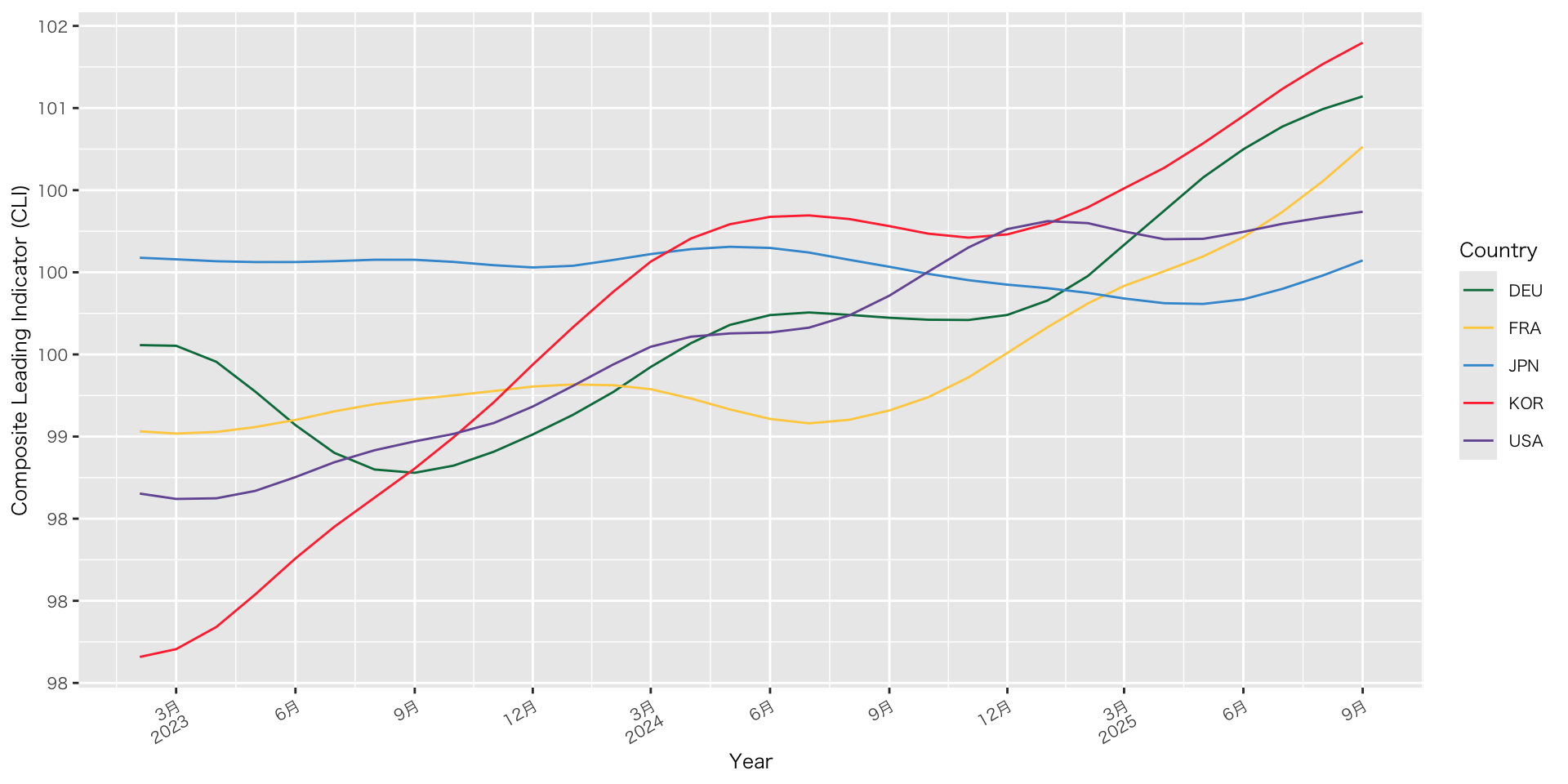
実践:ファイルの読み込み(訪日外客数の推移)
- データの読み込み:read_csv()関数
read.csv関数が補完入力されるかもしれません。read.csv関数はbase Rの関数で、今日では標準ではありません(.ドットと_アンダースコアの違い)
df_inbound <-
  read_csv("data/inbound_travelers.csv") # ファイル名は各自がつけたものとする

df_inbound |>
  ggplot(aes(x = Year, y = `Visitor Arrivals`)) + # カラム名に空白や記号が含まれている場合は、バッククォート(`)で囲む(日本語キーボード:Shift + @ / 英語キーボード:数字の1の左)
  geom_line() +
  scale_x_continuous(
    breaks = seq(1964, 2025, by = 5)  # 5年刻み
  ) +
  labs(x = "年",
       y = "訪日外国人客数") +
  scale_y_continuous(
    labels = label_number(big.mark = ",", accuracy = 1)
  ) # 指数表記を通常表記に(指数表記をあらためるためには、scalesパッケージを追加する必要があります)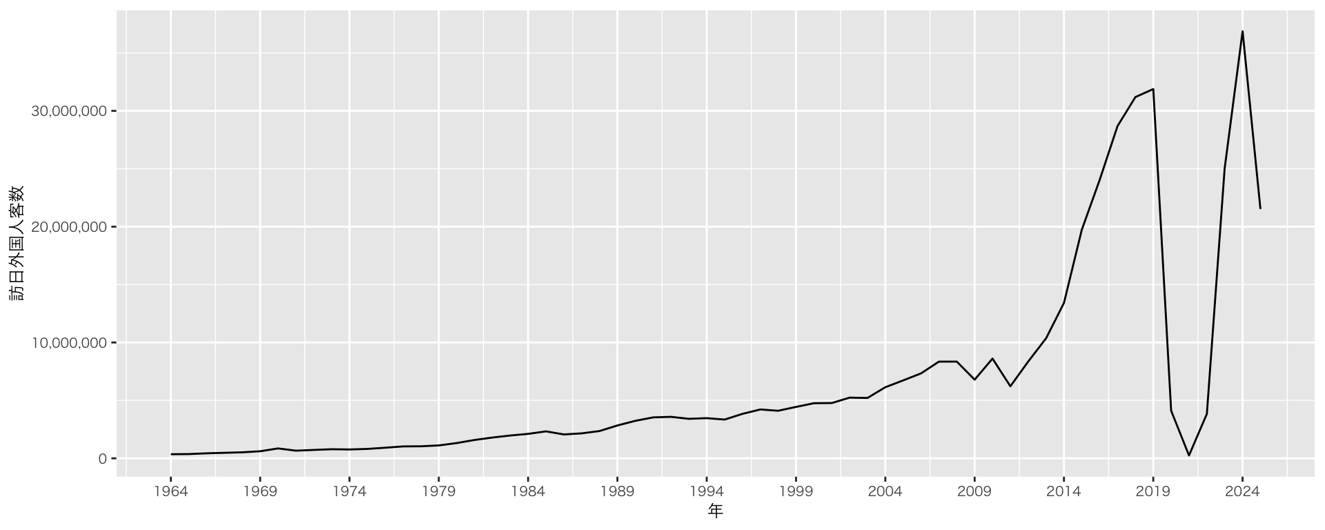
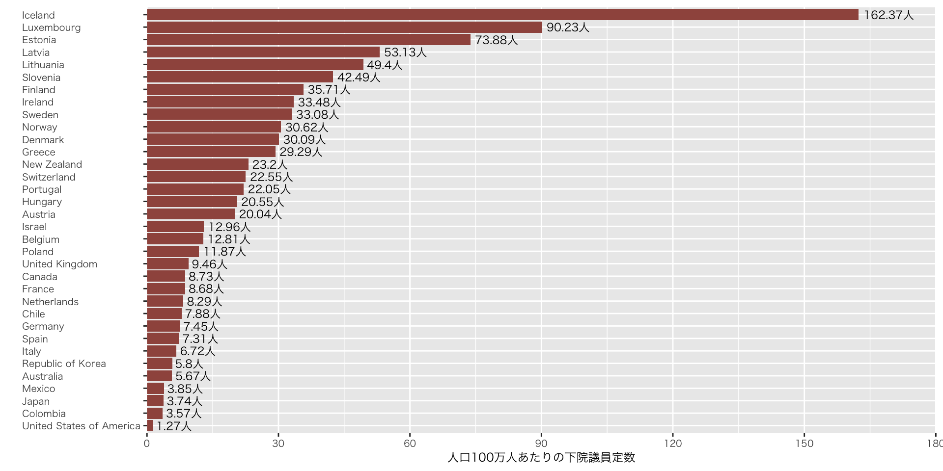
実践:データの結合(OECD加盟国の人口100万人あたりの議員数)
## 前処理(Setup Chunk)に書くべき

df_parline <-
  read_csv("data/parliaments.csv", skip = 15) # 冒頭から15行目まではメタデータ(ヘッダーコメント )なので読み込まない

df_population <- # ファイルが大きい(220.3MB)ため、重い処理かもしれない
  read_excel("data/population.xlsx", sheet = 1, skip = 16) |> # excelファイルはシートを指定できる
  filter(Type == "Country/Area") |>
  filter(Year == max(Year, na.rm = TRUE)) |>
  rename(country = `Region, subregion, country or area *`) # rename()でカラム名を変更

oecd_ISOcode <- c(
  "AU", "AT", "BE", "CA", "CL", "CO", "CR", "CZ", "DK", "EE", "FI", "FR",
  "DE", "GR", "HU", "IS", "IE", "IL", "IT", "JP", "KR", "LV", "LT", "LU",
  "MX", "NL", "NZ", "NO", "PL", "PT", "SK", "SI", "ES", "SE", "CH", "TR",
  "GB", "US"
)

oecd_countries <- c(
  "Australia", "Austria", "Belgium", "Canada", "Chile", "Colombia",
  "Czech Republic", "Denmark", "Estonia", "Finland", "France", "Germany",
  "Greece", "Hungary", "Iceland", "Ireland", "Israel", "Italy", "Japan",
  "Korea", "Latvia", "Lithuania", "Luxembourg", "Mexico", "Netherlands",
  "New Zealand", "Norway", "Poland", "Portugal", "Slovak Republic", "Slovenia",
  "Spain", "Sweden", "Switzerland", "Turkey", "United Kingdom", "United States of America", "Republic of Korea"
)

df_parline_oecd <-
df_parline |>
    filter(`ISO Code` %in% oecd_ISOcode) # %in% は複数の値をフィルタリングする際に使用〔特定の値の場合は==〕

df_parline_oecd <-
  df_parline_oecd |>
  # selectは文字通り列を選択する関数だが、選択する列名の前に「任意の名前 = カラム名」と書くことで、選択と列名の変更を同時に行うことができて便利
  select(country = Country, statutory_number = `Statutory number of members`)

df_population_oecd <-
  df_population |>
      filter(country %in% oecd_countries)

df_population_oecd <-
  df_population_oecd |>
  mutate(across(`0`:`100+`, as.numeric)) |> # 年齢に関する列がすべて文字列として認識されているため、across()で指定した列(0〜100+)をまとめて as.numeric() に変換する
  mutate(TotalPopulation = rowSums(across(`0`:`100+`), na.rm = TRUE)) |> # 年齢ごとの列(0歳〜100歳以上)の値をすべて足し合わせ、その合計を新しい列「TotalPopulation」に追加(欠損地は除外)
  select(country, TotalPopulation) |>
  mutate(TotalPopulation = round(TotalPopulation)) # TotalPopulation列の値を四捨五入して、整数に。結果は同じ列名TotalPopulation に上書き

df_pop_par <-
  df_population_oecd |> # df_population_oecdをベースに、df_parline_oecdを結合
  left_join(df_parline_oecd, by = "country") # countryをキーに

## 個別チャンク

df_pop_par |>
  mutate(
    statutory_number = as.numeric(statutory_number),
    member_per_million = statutory_number / (TotalPopulation / 1000),
    member_per_million = round(member_per_million, 2)
  ) |>
  arrange(desc(member_per_million)) |>
  mutate(country = factor(country, levels = country)) |> # 上記の順序で並べる(未指定だとアルファベット順に)
  ggplot(aes(x = fct_reorder(country, member_per_million),
             y = member_per_million)) + # fct_reorder() で棒グラフの順序をデータに合わせて並べ替え(未指定だと、逆順になる。ggplotの仕様)
  geom_col(fill = "#a0564d") +
  geom_text(                                     # 値を図に加える
    aes(label = glue("{member_per_million}人")), # 値に「人」を足す
    hjust = -0.1,
    size = 3.0
  ) +
  expand_limits(y = 180) + # Icelandの値がはみ出るため、x軸を180に
  scale_y_continuous(
    breaks = seq(0, 300, 30),
    expand = c(0, 0)
  ) +
  coord_flip() + # x軸とy軸を入れ替える
  labs(
    x = "",
    y = "人口100万人あたりの下院議員定数",
  ) +
  theme(
    axis.text.y = element_text(hjust = 0) # y軸のラベル名を左揃え(デフォルトは中央揃え)
) 
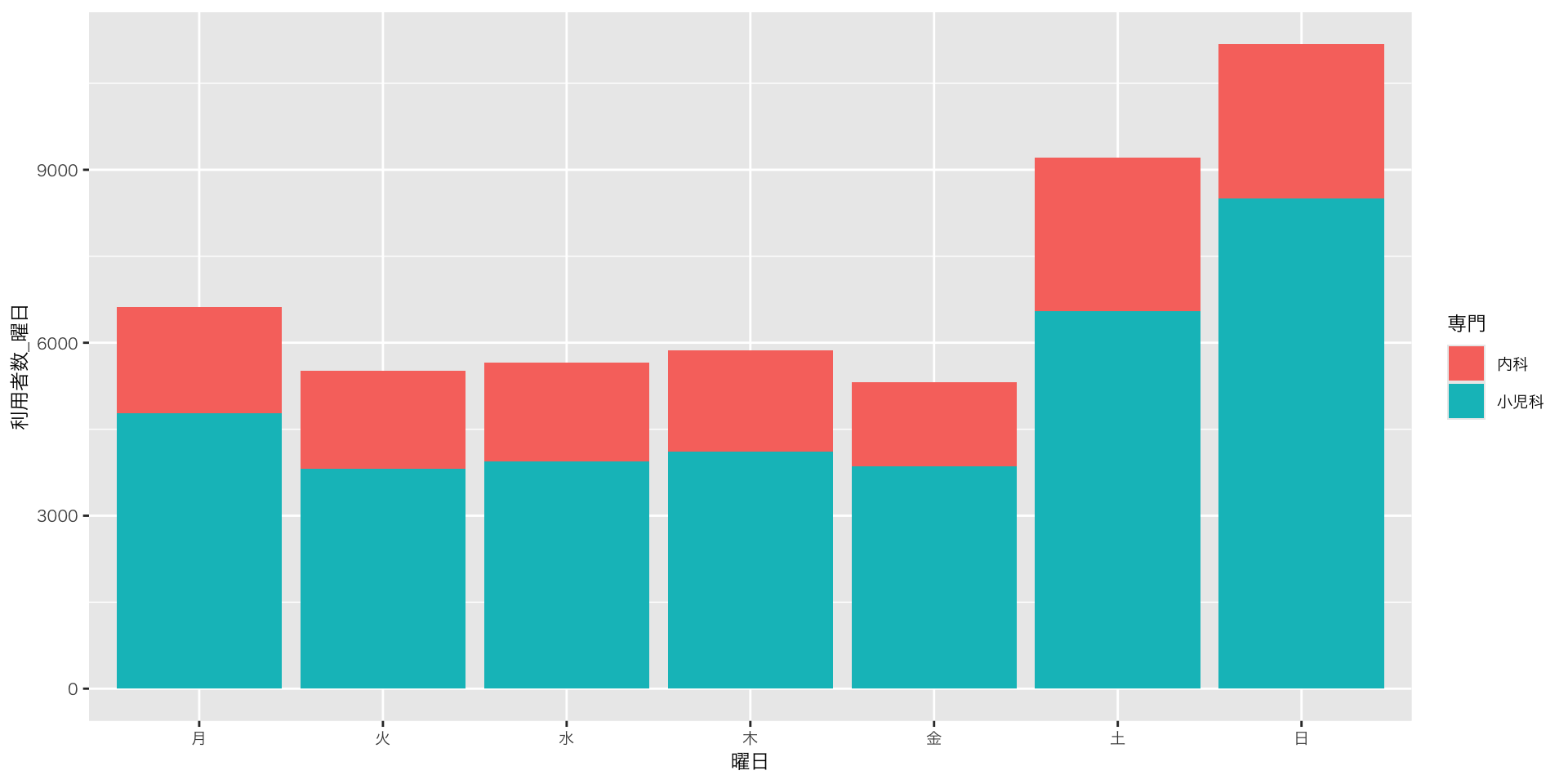
実践:縦持ち・横持ち(金沢広域急病センター利用者数)
縦持ちデータ(カラム「専門」)の活用
実践:比べられる図(比例代表得票数)
衆議院議員選挙 比例代表得票数:2021 vs. 2024
df_pr_parties |>
  group_by(year, party) |>
  summarise(
    votes = sum(votes)
  ) |>
  ungroup() |>
  filter(party %in% 主要政党) |>
  mutate(
    party = factor(party, levels = c("自由民主党", "立憲民主党", "公明党", "国民民主党", "日本維新の会", "日本共産党", "社会民主党", "れいわ新選組", "参政党"))
  ) |>
  ggplot(aes(x = party, y = votes, fill = as.factor(year))) + # yearをfactorにします(標準では数字です)
  geom_col(position = "dodge") + # 棒グラフを横並びにする
  scale_y_continuous(labels = zipangu::label_kansuji()) + # y軸のラベルをわかりやすくします(zipanguパッケージ要)
labs(x = "", y = "得票数", fill = "年") 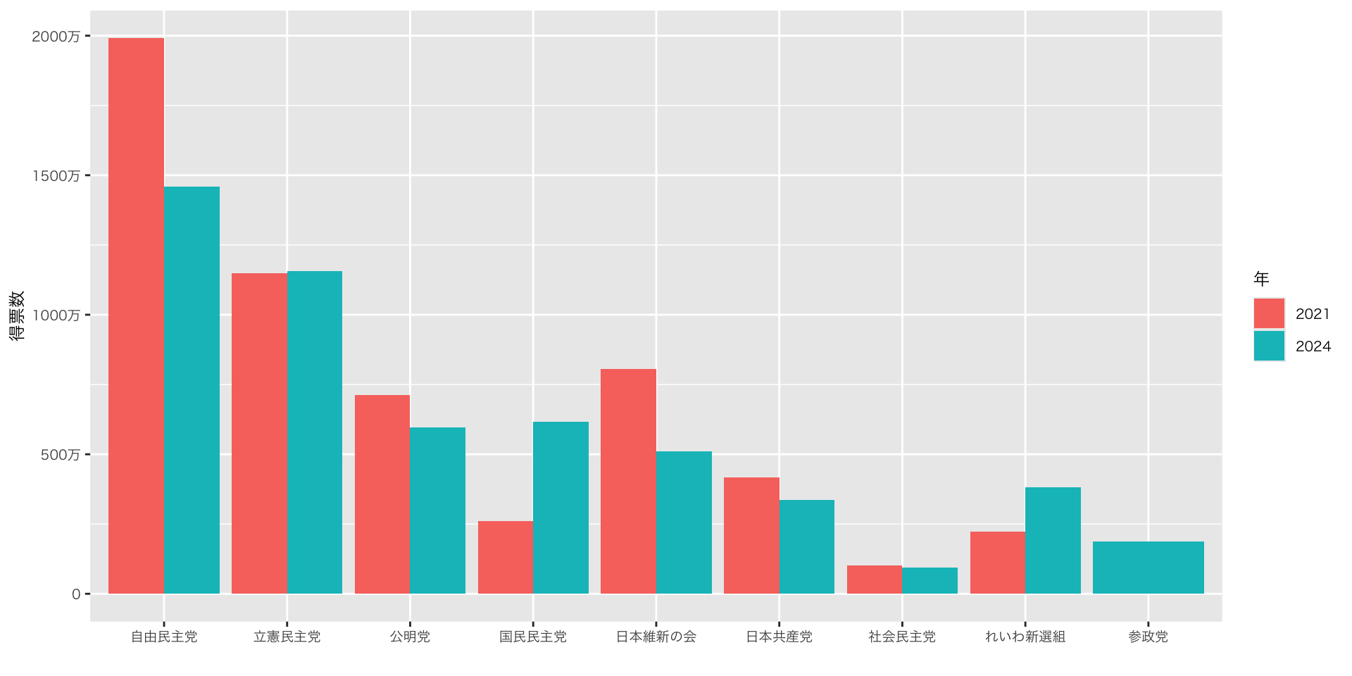
実践:比べられる図(比例代表得票数)
衆議院議員選挙 比例代表得票率:2021 vs. 2024
df_pr_parties |>
  group_by(year, party) |>
  summarise(votes = sum(votes), .groups = "drop") |>
  filter(party %in% 主要政党) |>
  mutate(
    party = factor(party, levels = c(
      "自由民主党", "立憲民主党", "公明党", "国民民主党",
      "日本維新の会", "日本共産党", "社会民主党", "れいわ新選組", "参政党"
    )),
    prop = votes / sum(votes)  # 各年で割合を計算
  ) |>
  ggplot(aes(x = as.factor(year), y = votes, fill = party)) +
  geom_col(position = "fill") +
  geom_text(aes(label = scales::percent(prop, accuracy = 1)),
            position = position_fill(vjust = 0.5), size = 3) + # 割合を中央に表示
  scale_y_continuous(labels = scales::percent_format(),
                     expand = expansion(mult = c(0.01, 0.01))) + # 左右のマージンを詰める
  scale_fill_paletteer_d("miscpalettes::brightPastel") + # 配色を変える
  labs(x = "年", y = "得票の割合", fill = "政党") +
  theme(legend.position = "bottom") + # 凡例を下に移動
  coord_flip() # 横向きに変える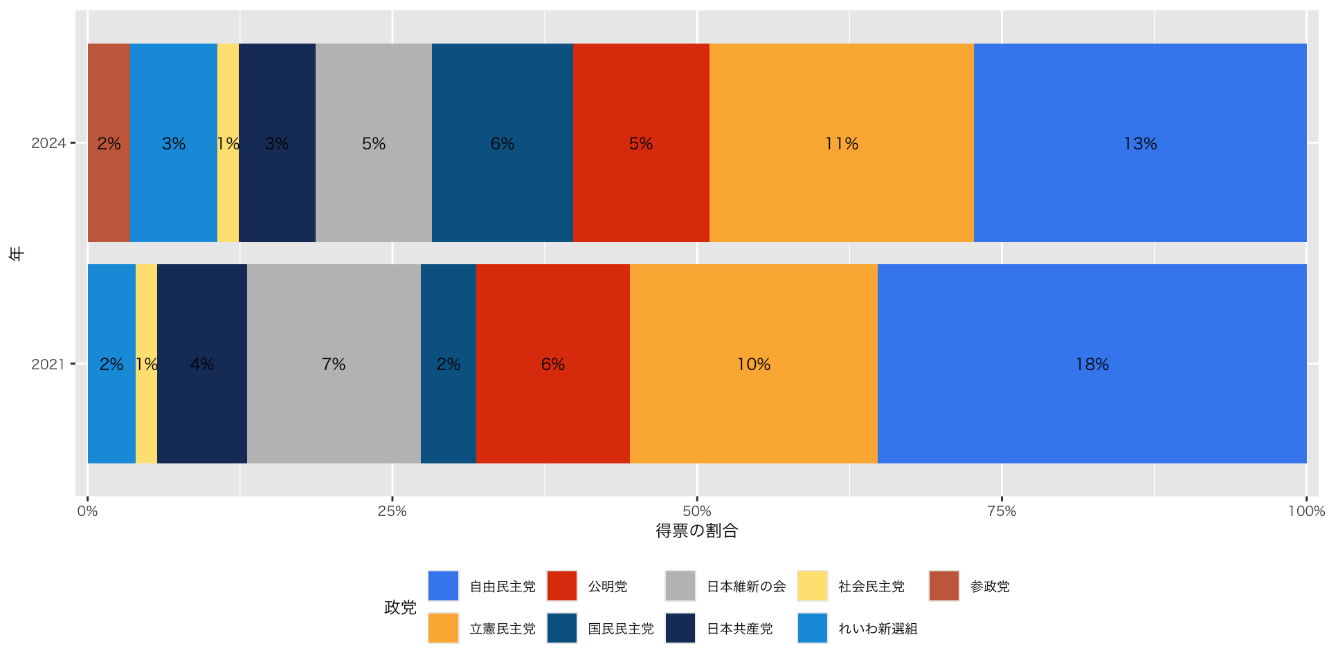
発展:地図情報(アメリカの選挙結果)
2016年アメリカ大統領選挙結果1
- ggthemesパッケージを使用
library(ggthemes)

us_state_elec |>
  ggplot(aes(x = long, y = lat, group = group, fill = party)) +
  geom_polygon(color = "gray90", size = 0.1) + # ggplot2内の関数
  coord_map(projection = "albers", lat0 = 39, lat1 = 45) +
  scale_fill_manual(values = party_colors) +
  labs(title = "アメリカ大統領選挙結果 2016", fill = NULL) +
  theme_map(base_family = "HiraKakuProN-W3") # 地図を描くときに余分な軸・枠・背景などを消して、地図表示に適したシンプルなテーマを適用する関数(注記・Windwowsユーザーはフォント変えて下さい)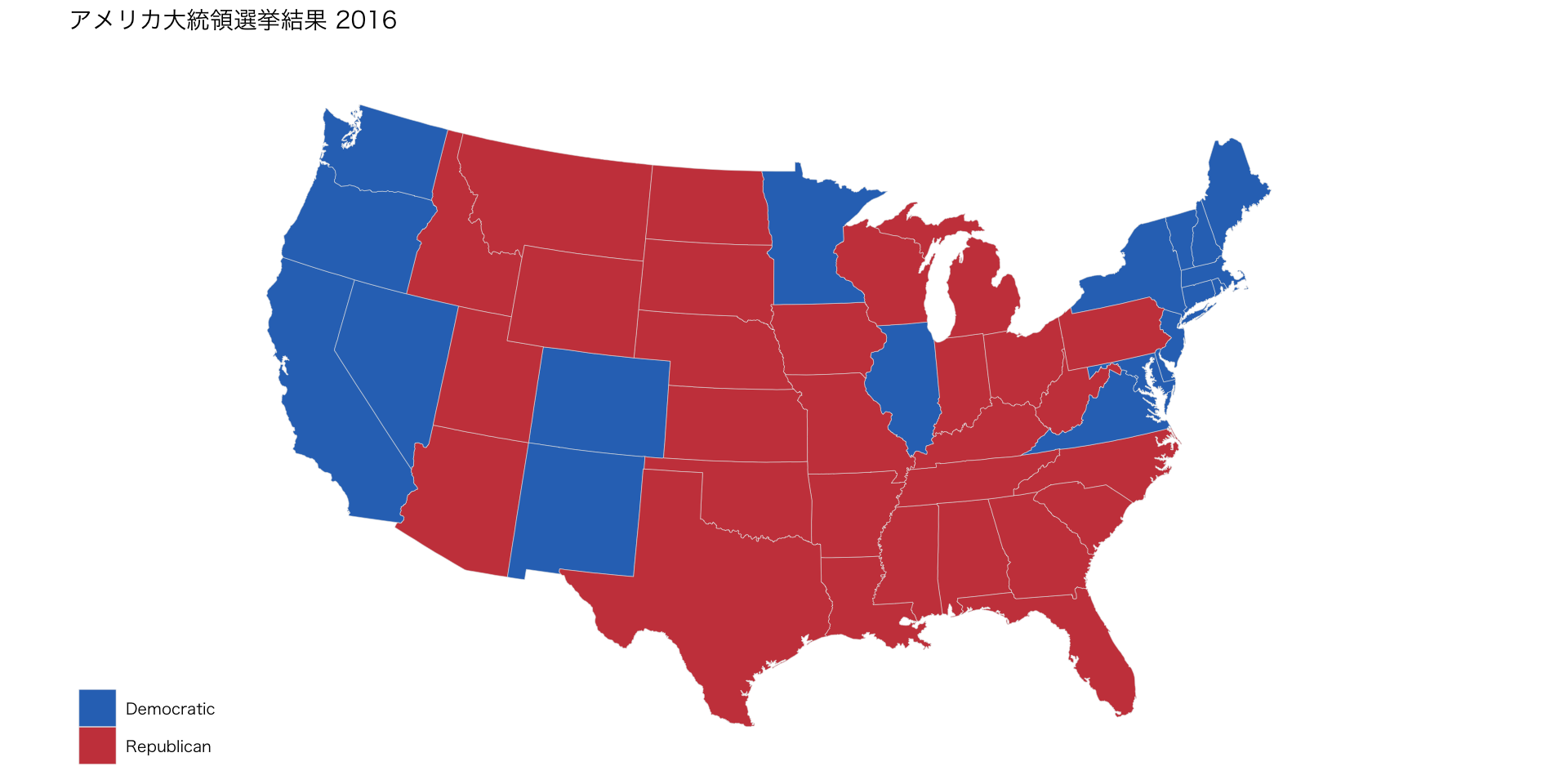
発展:地図情報(アメリカの人口密度)
アメリカの人口密度1
county_full <-
  county_map |>
  left_join(county_data, by = "id")

county_full |>
  ggplot(aes(x = long, y = lat,
         fill = pop_dens,
         group = group)) +
  geom_polygon(color = "gray90", size = 0.05) +
  coord_equal() +
  scale_fill_brewer(palette = "Blues",
                    labels = c("0-10", "10-50", "50-100", "100-500", "500-1,000", "1,000-5,000", ">5,000")) +
  labs(fill = "Population per\nsquare mile") +
  theme_map() +
  guides(fill = guide_legend(nrow = 1)) +
  theme(legend.position = "bottom")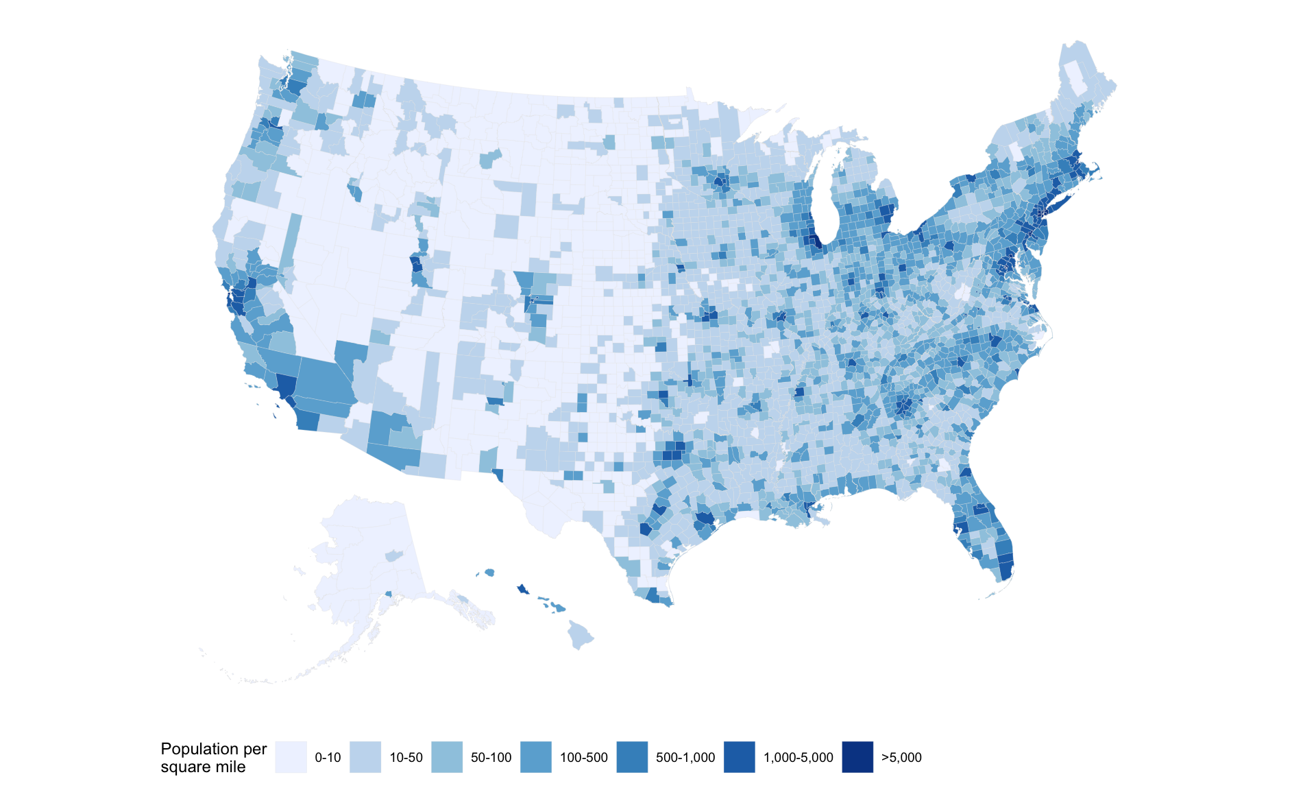
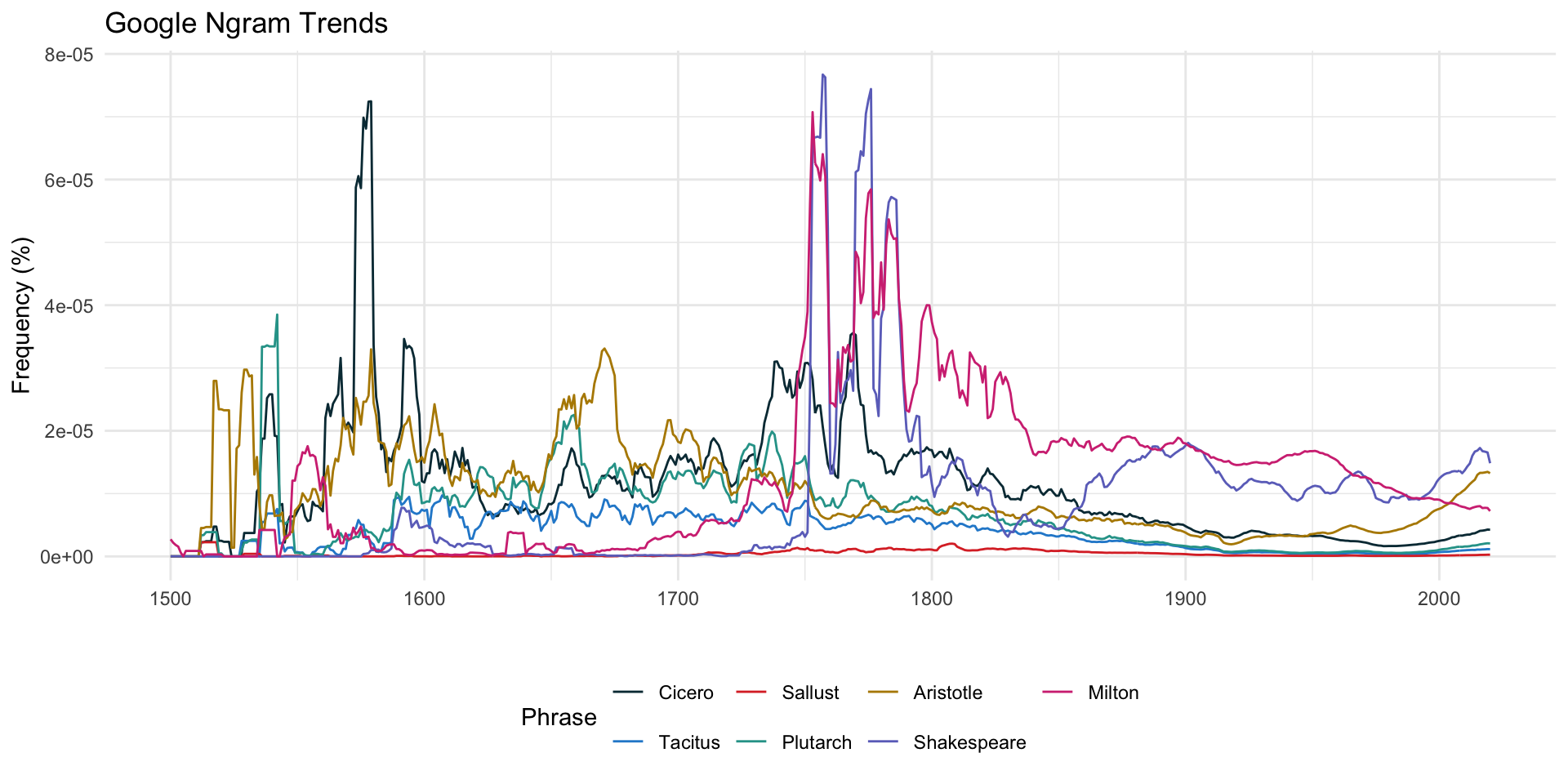
発展:Google Ngram Trends
- ngramrパッケージを使用
Code
library(ngramr)

words <- c("Cicero", "Tacitus", "Sallust","Plutarch", "Aristotle", "Shakespeare", "Milton")

df <- map_dfr(words, ~ngram(.x, corpus = "eng_gb_2019", year_start = 1500, year_end = 2020)) # 複数のオブジェクトに対して同じ処理を行い、その結果を 縦方向に結合(row-bind)してデータフレームにする

df |>
  ggplot(aes(x = Year, y = Frequency, color = Phrase)) +
  geom_line() +
  scale_color_paletteer_d("ggthemr::solarized") +
  theme_minimal() +
  theme(legend.position = "bottom") +
  labs(title = "Google Ngram Trends", y = "Frequency (%)", x = "")